COGITO Tutorials

These tutorials cover installing the COGITO code, running the main COGITO code, and analyzing bonding with the COGITO tight binding model. The workflow below provides the general outline. Click the section labels to quickly get to each section.

Workflow

Run VASP

A couple things to keep in mind for the VASP calculation:

Must be a static run (NSW=0)
Use an irreducible grid (ISYM=1,2,3)
Save the wavefunctions (LWAVE=True)
Use more bands (NBANDS=(8-16)*natoms)
No spin-orbit coupling (LSORBIT=False, but magnetism is supported (ISPIN=2)

Run COGITO

COGITO reads the INCAR, POSCAR, POTCAR, and WAVECAR files from the VASP calculation.

Step 1: Install COGITO
The COGITO code is not yet public, although it will be shortly. If you have access to the private repository, execute the code below to install COGITO and save its directly to the python path.

git clone https://github.com/olipemil/COGITO.git
# copy COGITO to python path
export PYTHONPATH="${PYTHONPATH}:/COGITO"

Step 2: Setup python environment
The following python packages can be pip installed:

pip install pymatgen
pip install matplotlib
pip install numpy
pip install scipy
pip install lmfit
pip install plotly
pip install seekpath
pip install dash

OR
For more reliable results, create a new conda environment for the yaml file in COGITO with conda

conda env create -f COGITO_env.yml

Step 3: Run COGITO!
The code below generates the COGITO basis and saves the tight binding model parameters in three files which will be used to initialize the next step.

tb_input.txt
TBparams.txt
overlaps.txt

from COGITO import COGITO

direct = "Si/"
# create an instance of the COGITO class
COGITOmodel = COGITO(direct) # set "spin_polar = True" for magnetic calculations
# do full algorithm and generate input files for TB model
COGITOmodel.generate_TBmodel(verbose = 0, plot_orbs = True, plot_projBS = True)

Run COGITO tight binding

Now we can work with our COGITO tight binding model. The first step is to verify the quality of the COGITO TB model.

Create the tight binding class
This code will need to be run before any use of the bandstructure or uniform classes.

from COGITOpost import COGITO_TB_Model as CoTB

direct = "Si/"
# create TB class from a directory that has run COGITO
my_CoTB = CoTB(direct)
# optionally, restrict the TB parameters to improve speed
my_CoTB.restrict_params(maximum_dist=15, minimum_value=0.00001)

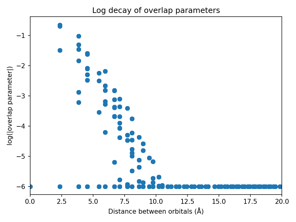
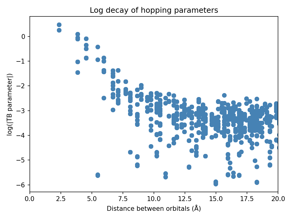
# plot the overlap and hopping parameters to check decay
my_CoTB.plot_overlaps(my_CoTB) # generates overlaps_decay.png
my_CoTB.plot_hoppings(my_CoTB) # generates tbparams_decay.png

Note: The overlap and hopping plots should show a rough linear decay

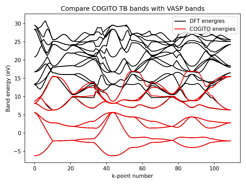
Compare COGITO band energies to DFT band energies
To verify the interpolation of COGITO, the function ‘compare_to_DFT’ is used to determine the error between the interpolating COITO band energies and DFT band energies. This function reads the DFT energies from an EIGENVAL file from a VASP (band structure) calculation.

# the EIGENVAL file you want to compare to
eig_file = my_CoTB.directory + "EIGENVAL"
# generates compareDFT.png and DFT_band_error.txt
[band_dist, max_error, band_error] = my_CoTB.compare_to_DFT( my_CoTB, eig_file)

Metrics for the fit quality will be printed and written to the DFT_band_error.txt as below.

File generated by COGITO TB
average error in Valence Bands: 0.006377 eV
band distance in Valence Bands: 0.011352 eV
max error in valence band: 0.053859 eV
average error in Bottom 3 eV of CB: 0.017887 eV
average error in Conduc Bands: 0.357561 eV

Run band structure class

This class generates the band structure for high symmetry path determined with pymatgen. Importantly, this class requires an instance of the tight binding class in initialization.

# must create TB class instance first
from COGITOpost import COGITO_TB_Model as CoTB
direct = "Si/"
my_CoTB = CoTB(direct) # create TB class from a directory that has run COGITO
my_CoTB.restrict_params(maximum_dist=15, minimum_value=0.00001) # restrict the TB parameters to improve speed

# now create band structure
from COGITOpost import COGITO_BAND as CoBS
my_CoBS = CoBS( my_CoTB, num_kpts = 10) # num_kpts is actually num per line, so set low
# optionally, plot band structure
my_CoBS.plotBS()

Use COGITO for orbital projected band structure
Because COGITO forms a nearly complete basis for the charge density, we can accurately determine the percent of each atomic orbital in the band wavefunction. Mulliken population analysis is used here to resolve the inherit ambiguity in assigning two-center terms to one orbital.

# plot the projected band structure of Si s orbitals
my_CoBS.get_projectedBS({"Si":["s"]})

Use COGITO for COHP/COOP projected band structure
The accurate TB model from COGITO allows for calculation of COHP energies which almost perfectly reflect the true DFT values. This can be used to confidently and precisely trace back the crystal chemical origins of electronic structure!

Any COHP requires specifying two sets of orbitals. The bonds between any orbital in set 1 with any orbital in set 2 is included in end COHP.

# specify the two sets as a list of two dictionaries
# in the dictionary, the keys are elements, and the values are the orbitals included for that atom
# each dictionary can have multiple atoms as keys
orbs_dict = [{"Si":["s","p","d"]},{"Si":["s","p","d"]}] # for silicon
#orbs_dict = [{"Pb":["s","p","d"],"O":["s","p","d"]},{"Pb":["s","p","d"],"O":["s","p","d"]}] # for PbO
my_CoBS.get_COHP(orbs_dict)

# bonus points for running the interactive dash app
# this populates the autogenerates options for orbs_dict for the user to choose from
my_CoBS.make_COHP_dashapp()

Run uniform class

Last, but not least, this class works with a uniform grid of k-points. The uniform grid gives us access to integrated properties like: atomic charge, covalent bond energy (ICOHP), projected density of states (DOS), etc.

Like the band structure class, the uniform class requires the input of a TB class instance.

# must create TB class instance first
from COGITOpost import COGITO_TB_Model as CoTB
direct = "Si/"
my_CoTB = CoTB(direct) # create TB class from a directory that has run COGITO
my_CoTB.restrict_params(maximum_dist=15, minimum_value=0.00001) # restrict the TB parameters to improve speed

# now create band structure
from COGITOpost import COGITO_UNIFORM as CoUN
my_CoUN = CoUN(COGITOTB,grid=(10,10,10))
my_CoUN.get_occupation()

Running the get_occupation function prints the output below. The first line shows how many electrons are in each orbital with Mulliken population analysis. The second line ‘sum’ should be the total number of valence electrons. The third line is the electrons in each orbital without Mulliken. The final line is the electrons for each atom with Mulliken population analysis.

Where are the electrons?
orbital + overlap occupation: [1.36334891 0.87881112 0.87891999 0.87891997 1.36334891 0.87881113 0.87891997 0.87892   ]
sum:  8.0
orbital occupation without bonds: [1.09389053 0.56850573 0.56864044 0.56864041 1.09389055 0.56850573 0.56864041 0.56864043]
The electron occupation for the atoms  ['Si' 'Si']  is  [3.99999999 4.00000001]

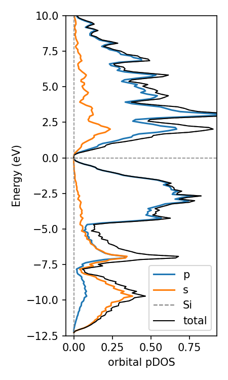
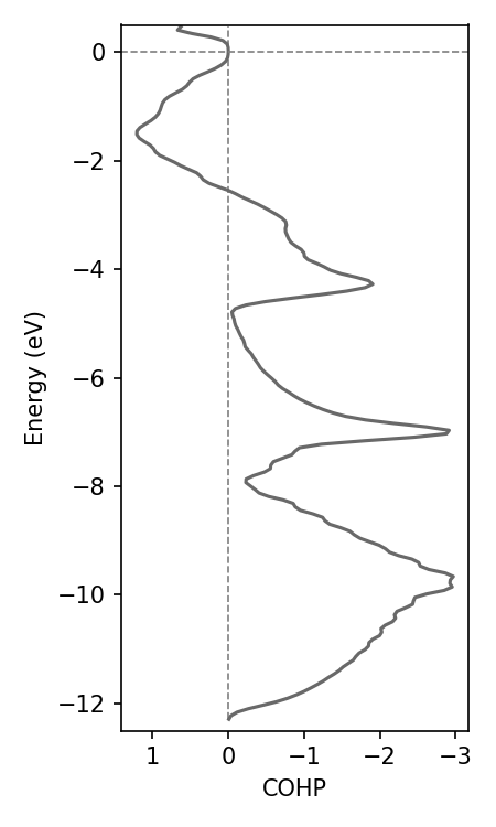
Use COGITO for orbital/COHP/COOP projected DOS
Because COGITO forms a nearly complete basis for the charge density, we can accurately determine the percent of each atomic orbital in the band wavefunction. Mulliken population analysis is used here to resolve the inherit ambiguity in assigning two-center terms to one orbital.

Any COHP requires specifying two sets of orbitals. The bonds between any orbital in set 1 with any orbital in set 2 is included in end COHP.

# Get orbital/element projected DOS for an element
my_CoUN.get_projectedDOS("Si",ylim=(-10,5),sigma=0.09) # sigma is gaussian smearing, adjust with initial k-grid

# specify the two sets as a list of two dictionaries
# in the dictionary, the keys are elements, and the values are the orbitals included for that atom
# each dictionary can have multiple atoms as keys
orbs_dict = [{"Si":["s","p","d"]},{"Si":["s","p","d"]}] # for silicon
#orbs_dict = [{"Pb":["s","p","d"],"O":["s","p","d"]},{"Pb":["s","p","d"],"O":["s","p","d"]}] # for PbO
my_CoUN.get_COHP(orbs_dict)

Use COGITO to plot crystal bonds!

The accurate TB model from COGITO allows for calculation of COHP energies which almost perfectly reflect the true DFT values. This can be used to confidently and precisely trace back the crystal covalent bonding!

# must create TB class instance first
from COGITOpost import COGITO_TB_Model as CoTB
direct = "Si/"
my_CoTB = CoTB(direct) # create TB class from a directory that has run COGITO
my_CoTB.restrict_params(maximum_dist=15, minimum_value=0.00001) # restrict the TB parameters to improve speed

# now create band structure
from COGITOpost import COGITO_UNIFORM as CoUN
my_CoUN = CoUN(COGITOTB,grid=(10,10,10))

# plot the crystal structure with real bonds!
# if a bond energy magnitude is > energy_cutoff it will be plotted
# if the bond length is > bond_max it will not be plotted if an atom is outside the primitive cell 
my_CoUN.get_bonds_figure(energy_cutoff=0.05,bond_max=3)